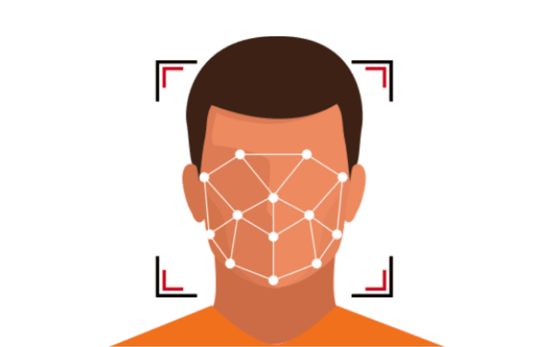
Humans have an amazing ability to recognize faces, and artificial intelligence algorithms are slowly matching these capabilities.
There is no simple explanation for how humans perform this common cognitive task, which is often referred to “face perception.” Face perception involves a network of neural pathways stretching from the eyes to the fusiform face area of the brain, though a precise understanding of the face perception process is currently beyond our reach [1]. Of course, despite the fact that most people don’t understand the underlying biological mechanisms used by their brains to identify a face, most everyone can identify a face without much issue.
In many ways automated face recognition is just as complicated as human face perception. The precise techniques employed by automated algorithms are often nuanced, dependent on machine learning techniques that are difficult to explain, highly computational, subject to trade secret if commercial, and often lacking in reproducibility if academic. Fortunately, an understanding of these nuanced techniques is not required to distinguish the strengths and limitations of a given face recognition (FR) algorithm or to use it effectively. However, a basic understanding of how automated FR algorithms function can be quite helpful to properly work with them.
This article offers a high-level guide to how automated face recognition algorithms work, targeted to integrators of face recognition libraries and those seeking cursory insight into how this cutting edge technology is developed.
The Two Steps for Automated Face Recognition (FR)
There are two primary steps repeatedly performed when using automated FR technology. The first step is to detect a face within an image and represent the measurements of key facial features of the detected face, which is collectively referred to as “representation” or “enrollment.” The second step is comparing two or more of these representations in order to determine their facial similarity, which is referred to as “comparison” or “matching.”
A well-designed face recognition API will allow these two key tasks to be performed in just a few function calls, while having several additional helper functions and parameters to handle all the different aspects of a particular application. Our deeper dive into these two processes below will help you understand the parameters typically involved.
Representation
The representation step is used to process all incoming imagery. This could be from the initial ingestion of a reference database of images (e.g., employee ID card images), or during a live presentation of a face to the system (e.g., an employee presents themself to a camera for facility access). The output of the representation step is a facial template that contains the encoded facial features.
The steps performed during representation, to go from an input image to encoded facial features, are as follows:

Face Detection
The first step in automated face recognition is to detect all faces present in an image. In some cases the application may dictate that there will only be one face in an image (e.g., capturing ID card photo), but unless the integrator provides this information to the algorithm, the algorithm cannot make any such assumptions. Instead, it will attempt to detect all faces present in an image (or video frame).
Let’s consider the following image as an example:
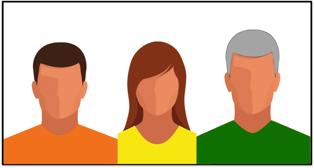
After performing the face detection step, an algorithm should accurately determine the location of all faces present:

However, it could be the case that a non-face region is incorrectly detected as being a face:

Or, it could be the case that one of the actual face regions is not detected:
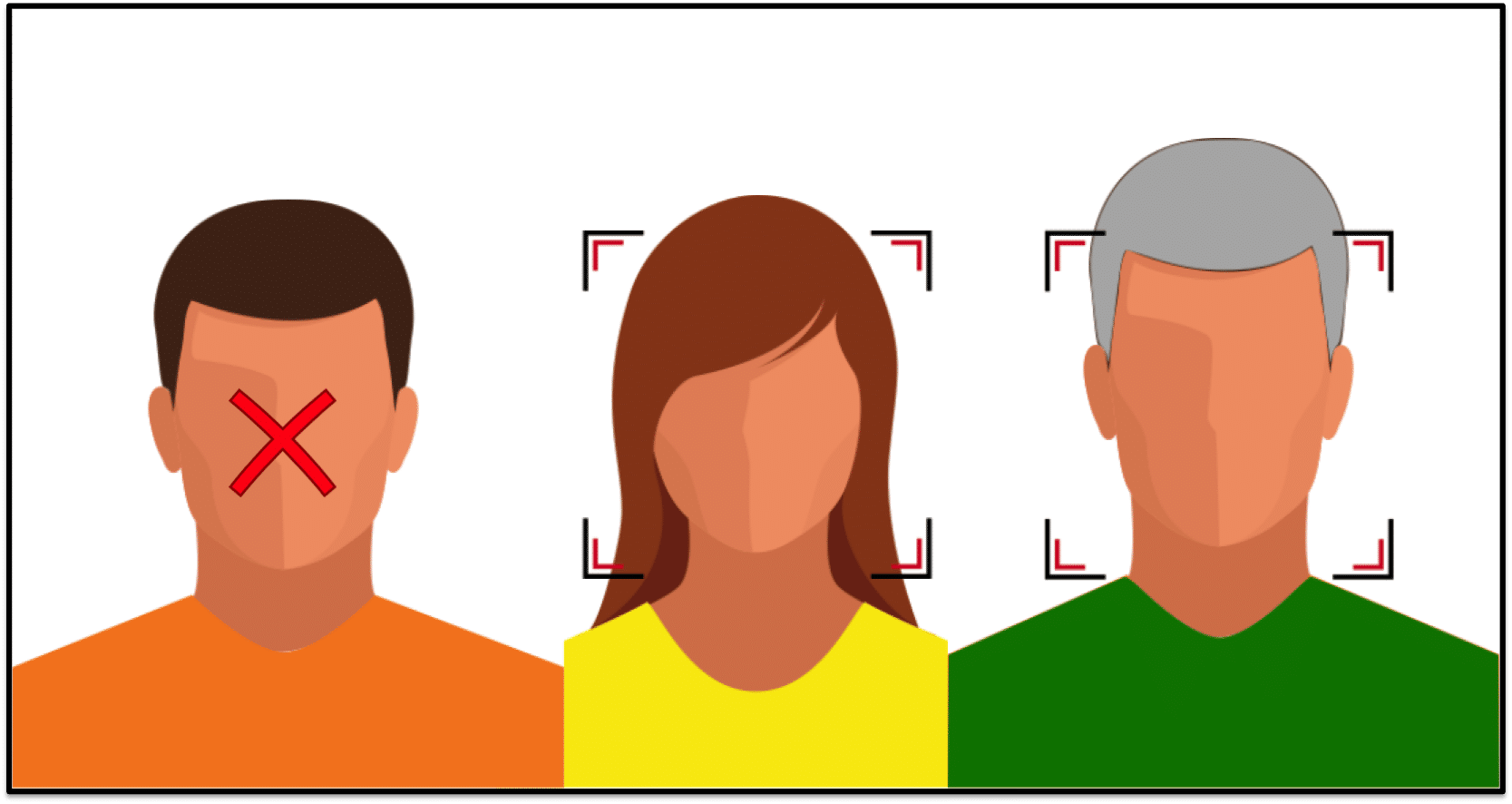
For controlled environments face detection is typically near-perfect, but it is important to consider the implications of the two types of error cases that are illustrated above as they will eventually happen to even the best face detection algorithms.
When a face is not detected (false negative), there is obviously no chance to recognize it. Thus, this error case can undermine the intent of the system. When a non-face is incorrectly detected as a face (false positive), this causes the system to further process the non-face region as if it were a face. Depending on the configuration of the system, at best this will result in wasting system resources. At worse this will result in a person’s claimed identity being stored in a database with a non-face region as opposed to their actual face region.
A well-designed face detection API exposes a detection confidence threshold which adjusts the likelihood of false positives and false negatives. Lowering the threshold results in more false positive detections and fewer false negative detections. Conversely, raising the threshold results in fewer false positive detections and more false negative detections. Your application will dictate which one of these scenarios is more desirable for your system. Typically the default threshold will be appropriate to use.
Now, you might be asking, how does the face detection algorithm attempt to determine where the faces are in the first place? The answer is rather rudimentary: a brute-force inspection of every possible region in the image is performed. This approach is often referred to as a “sliding window.” A sliding window will consider all different image locations, and all different face sizes, and for each scale and location pass the region being inspected into a classifier to decide whether or not that region is a face.
To illustrate how a sliding window works, let’s consider the following image with two faces present at different distances from the camera:

To find the faces in this image the sliding window will first start by considering the largest face bounding box size possible:
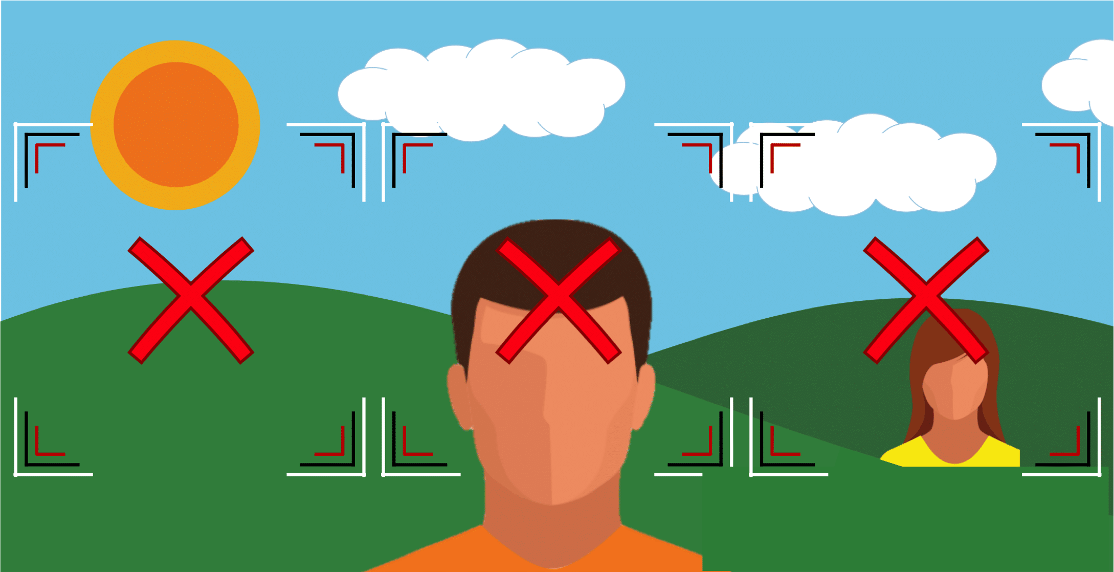
As no faces match this bounding box size, no faces are detected in this pass. In the next pass, the bounding box size will be decreased, and all potential locations at this scale will now be considered:
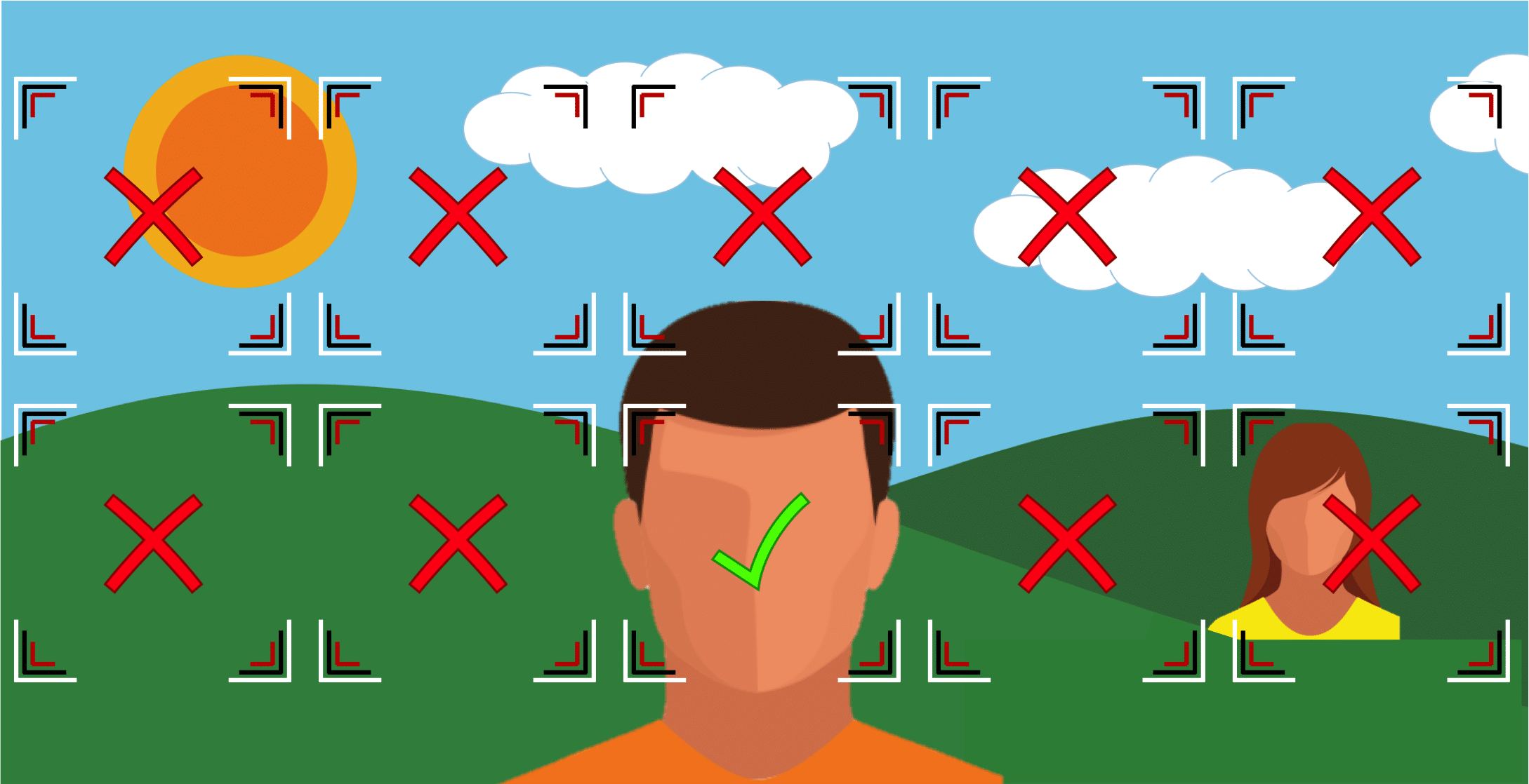
In this case, one of the faces is detected. And, this process continues with the bounding box continuing to decrease and all regions at that scale being inspected:

The process ends when the face bounding box size is less than the minimum value specified by the software. This minimum bounding box size is typically a user-adjustable parameter.
As the simple illustrations above demonstrate, the smaller bounding box sizes will result in an exponentially larger number of candidate regions to consider. Thus, knowing the proper minimum bounding box size can save a lot of computation time.
The above examples ignore a few key considerations. First, the bounding boxes considered by the sliding window process will overlap quite a bit in practice. Second, the successive decreases in bounding box scales will typically reduce the bounding box size by roughly 25%. Many other nuances are involved, but the illustrations above do capture the key concept of how faces are found in an image.
How a given region is determined to be a face or a non-face is beyond the depth of this article, but readers with a deeper curiosity should read the “Viola Jones” research paper [2]. This face detection algorithm was groundbreaking in the field of face detection when published 15 years ago, and in many regards it is still relevant today.
Feature Localization
Once faces have been detected the algorithm next needs to understand where the different features of the face exist. That is, because the face is a highly rigid structure (we have two eyes that are above a nose, our nose is above our mouth, etc.), the algorithm can benefit tremendously from refining its understanding of precisely where different parts of the face reside within a detected face region. Of course, while some algorithms choose to bypass this step in its explicit form, this localization process is still implicitly performed during subsequent representation extraction.
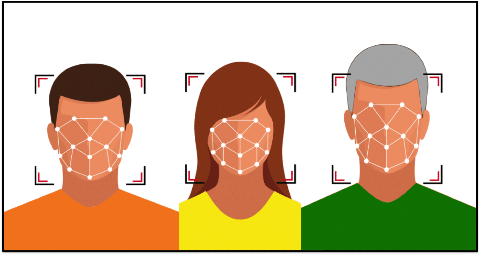
For many algorithms the localization step is a key area where accuracy can degrade. For example, many times off-pose face images (i.e., faces not looking towards the camera) may fail to localize properly by algorithms that have not been developed for such conditions.
Many face recognition algorithms will expose certain artifacts of the localization step that can be useful for determining if a failure occurred during this step. For example, it is common to output the location of the center of the eyes. If the coordinates output are incorrect it is likely that the localization caused the algorithm to fail.
Representation
After feature locations are firmly established for a face, the algorithm next performs complex measurements that describe the structure, appearance, and relationship of the different facial features. This step can be referred to as “representation,” and the specific techniques applied vary significantly across algorithms. While earlier approaches used manually specified feature measurements, modern day methods prefer measurements that are derived from machine learning algorithms.
One of the most common misconceptions about face recognition is that the algorithms explicitly measure distances between the eyes, nose, and other features in the face, and then use these anthropometric distances and ratios to determine the similarity of two faces. While some early attempts at face recognition used this approach (e.g., several decades ago in computerized form and over one hundred years in the Bertillon System), such measurements lack proper discriminability to perform identification across any meaningfully sized population.
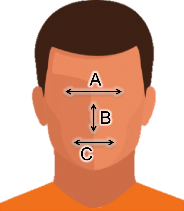
Face recognition does not explicitly measure distances across the face. Such simple measurements cannot accurately distinguish identity.
The earliest automated algorithms to gain any form of reasonable success represented a face based on localized pixel intensity values, where localized refers to faces or face regions being canonicalized from the previous localization step. Because each pixel is (typically) a value ranging from 0 to 255 (after being converted from color to grayscale), early algorithms used the values of these pixels to directly represent the face. Though limited success was achieved with this approach [3], pixel values will change drastically amid variations in illumination or facial pose, thus rendering this technique insufficient in practice.
![]()
Representing a localized face with pixel values is how many early face recognition systems operated and achieved mild success.
One of the major breakthroughs in face recognition representations was using “texture patterns” to represent the face. Born out of the methods formalized in the computer vision literature from the 80’s and 90’s, texture patterns measure higher order relationships between neighboring pixels. Thus, instead of simply using the pixels to represent the face, the structured differences between neighboring pixel values were measured. The chief benefit of using these texture patterns is that they naturally describe the curvatures of the face while being less affected by variations in lighting and capture conditions.
Some of the common texture methods popularized in face recognition algorithms from the late 90’s and early 2000’s, which have generally persisted in many commercial algorithms until the last several years, used techniques such as Gabor filters [4] (which convolve sinusoidal waves against the image intensity / pixel values), local binary patterns (LBP) [5] (which encode the relative differences between neighboring pixel values into histograms of pattern-types), and histogram of oriented gradients (HOG) [6] (which measures the direction and intensity of pixel changes and coarsely bins them into a histogram). All of these approaches are all able to capture the structure of the face amid certain environmental changes and thus enable good face recognition accuracy in certain conditions.
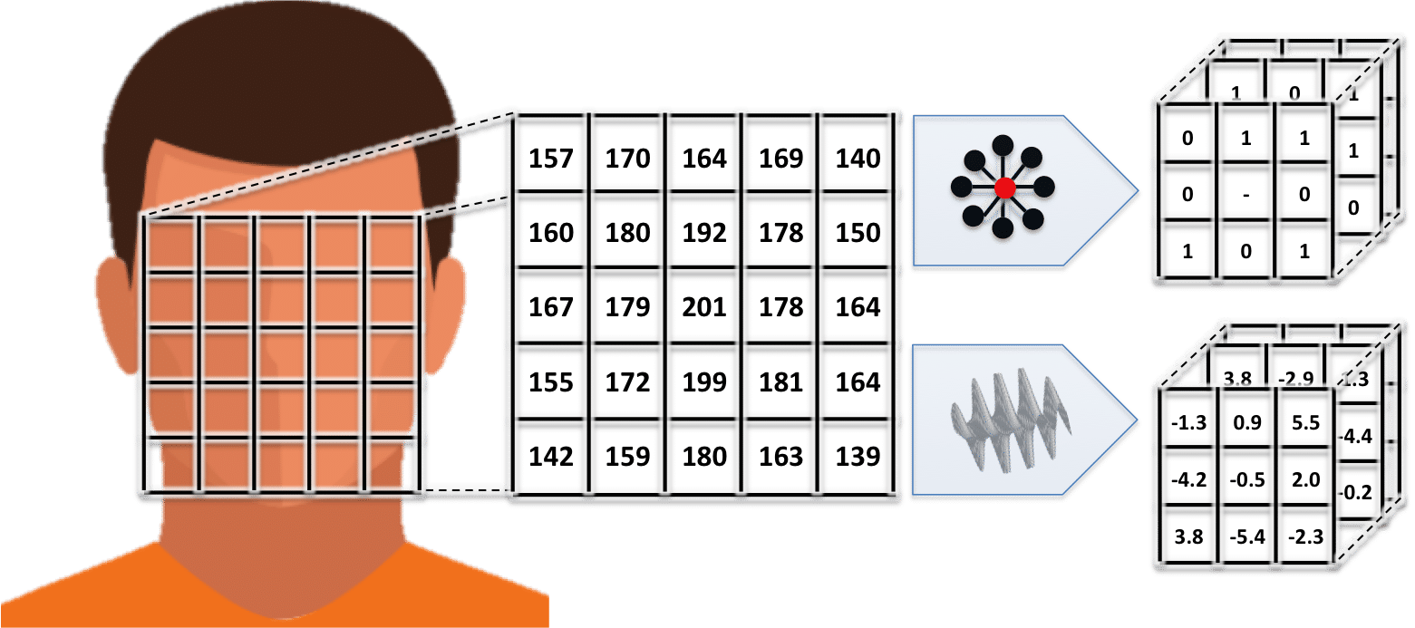
Despite a long run of success at constrained face recognition tasks, texture-based face representations never achieved meaningful success on unconstrained face recognition tasks.
Texture based methods such Gabor, LBP, and HOG, along with various machine learning techniques that are often applied in conjunction, enabled the first operationally successful face recognition systems. These systems were generally successful when matching constrained face images, which are images where the environment is controlled and the person being photographed is cooperating (e.g., visas and mug-shots). However, these representations still failed in the most challenging conditions (e.g. large facial pose and illuminations variations, and occlusions) and lacked precision when operating on large-scale constrained databases.
The major breakthrough in the last few years, which has catapulted face recognition algorithms from limited use-cases to the vast range of applications that are now emerging in the marketplace, was advancement in deep learning [7] and convolutional neural networks (CNN’s) [8]. Some key differences between CNN’s and higher order features is that while Gabor, LBP, and other similar approaches used relatively simple “hand-coded” techniques to measure the structure of the face (i.e., the measurements by each technique are manually developed in software by a person), CNN’s learn the measurements to perform automatically and with orders-of-magnitude more depth and complexity. Thus, while Gabor and LBP may be effective in certain scenarios, they are not necessarily optimal for the task at hand.
When attempting to learn a CNN representation for use in automated face recognition, the deep learning frameworks (e.g., Caffe or TensorFlow) will be prescribed an architecture from the algorithm developer which dictates how information, starting from the image pixels, flows through the network. This includes the size, type, and number of the different convolutional filters learned (which can capture the spatial relationships across the image or within the latent feature representations inside the network), where to apply feature pooling (which effectively downsamples the filter responses), how to linearly combine these features into a compact representation (to enable classification), and other more advanced considerations.
Despite all these immense considerations when designing a network, the values of the filters and feature weights are learned by the framework itself. This learning is performed using large face image datasets and it can take several days to weeks to train a “deep” network.
It is not uncommon for a CNN architecture to result in hundreds of millions of computations to extract the representation of a face. The power of learning a representation based on so many calculations should be evident both from the sheer difference in the amount of computations used with a CNN as compared to earlier representations, as well as with tremendous improvements in face recognition accuracy that have been observed in recent years. However, with this increased complexity comes many additional considerations for developers. For one, the amount of training data required is significantly larger than other methods, as is the amount of time required to train the algorithm. Further, mis-calculating the amount of training data required relative to the architecture being used can result in a representation that is highly overfit to the training data. In turn, this representation will not perform well on data that does not closely match the training data.

In a basic Convoluational Neural Network (CNN) network raw pixels are passed through layers of convolutional filters, pooling, and feature weighting.
Templates
While a wide range of representations have been discussed, regardless of the technique performed, the representation will typically result in a fixed-length numerical vector, referred to as a “template,” which is the final representation of the characteristics of a face; the “faceprint,” as some have called it. The benefit of representing a face this way is that it enables simple and rapid comparison.
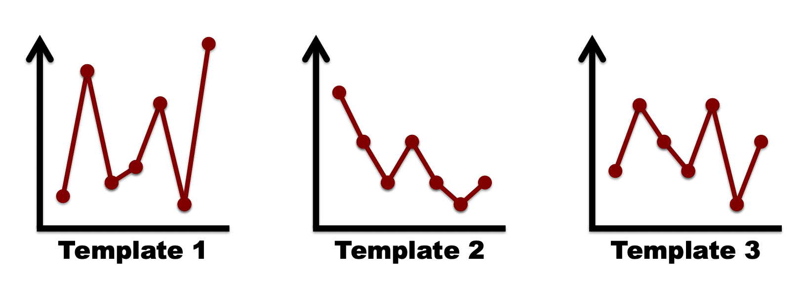
The final template used to represent a face is a point in a high-dimensional space. Two templates can be compared using various distance metrics.
Enrollment
The process of performing face detection, localization, and representation to produce a template is collectively referred to as “enrollment.” This term is commonly used when discussing the enrollment speed of a given algorithm, which is the time it takes to ingest an image and output a template for each detected face. Enrollment speed is typically measured on a single CPU core as it is trivial to parallelize the enrollment of multiple images across multiple CPU cores. Industry enrollment speeds generally range from 50ms to 1s [9], and thus the number of CPUs required for a given application can fluctuate significantly depending on the algorithm.
The size of the templates produced by the enrollment process will also vary significantly depending on the algorithm. For example, industry template sizes currently range from about 100 bytes to 64,000 bytes [5]. Template size impacts the amount of computer memory that is needed to cache the templates for rapid access during comparison, as well as the amount of processing required to perform a comparison.
Different representations are generally going to have different degrees of robustness and relevance to different environmental factors. However, understanding what specific representation is used in a given method does not provide any meaningful advantage to a user of that algorithm.
As third-party benchmarking of commercial face recognition algorithms often attests [9], algorithms from different vendors, having vastly different implementations, often fail in similar conditions. This leads to the following important concept: regardless of the particular issue that a given representation may suffer from, an end-user of the algorithm only needs to know that the issue exists, and not as much why the issue exists.
Given the importance of simply understanding that an issue exists, note that a pending article [cite] will provide guidance on how to evaluate the accuracy of face recognition algorithms and understand if any such issues exist.
Comparison
Once faces are represented as templates they can in turn be compared to determine their similarity.
End-users of a face recognition system will generally only observe the output of the comparison step in terms of “match” or “no match.” This is because the system received a similarity score between the two or more faces and decided if they are the same person or different based on a threshold of the numerical similarity score.
Together with documentation on how to assess the significance of different similarity scores (as well as internal benchmark datasets, a topic that will be discussed in a forthcoming article) integrators and users will be able to make actionable use of the similarity score produced by comparing two templates.
The process for measuring the similarity score is as follows:
1. Generate the template for each face image:
2. Measure the similarity score:

Typically there are two different reasons to perform template comparisons:
- To determine if two face images (via their templates) are the same person or different. This is often referred to as one-to-one (1:1) identity verification
- Determine the identity of a given face image / template using a database of face images (a gallery of templates) as a reference. This is often referred to as one-to-many (1:N) identification.
1:1 Identity Verification
When performing “one-to-one (1:1) identity verification” the comparison process is straightforward. The two templates are the input into the comparison function provided by the face recognition algorithm and the similarity score is the output. Typically a similarity threshold has been determined by the integrator in advance, and if the similarity of the two templates exceeds the threshold they are considered to be a match (same person), otherwise they are considered to be a non-match (different person). Depending on the degree of human operation for a given system, certain scores near the threshold may be sent to a human for manual review.
The following example illustrates how the thresholding process works for two different template comparisons. In this example the maximum similarity score is 1.0 and the minimum similarity is 0.0, however in practice a given face recognition algorithm may span any numerical range.
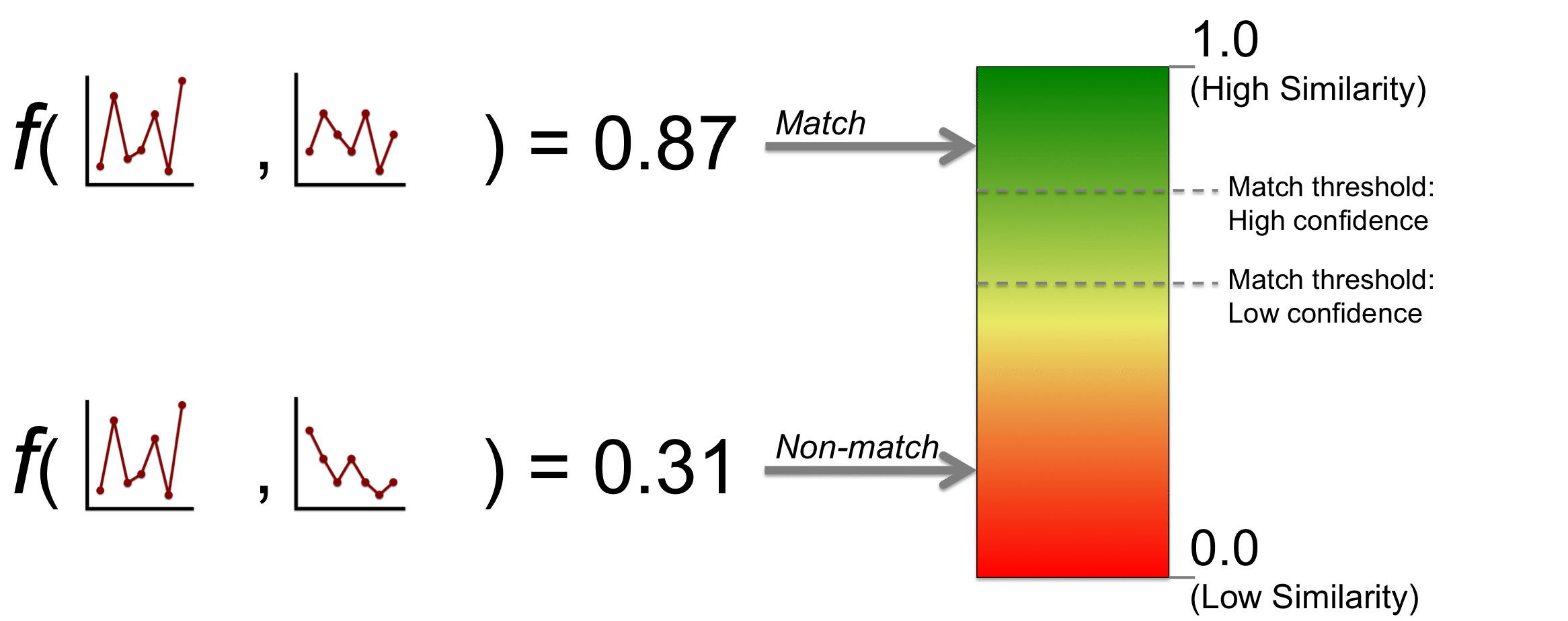
When two templates are correctly determined to correspond to the same person, this a known as a “true accept.” When two templates are correctly determined to correspond to different persons, this is known as a “true reject.” When two templates are incorrectly determined to correspond to the same person (and are actually different persons), this is known as a “false accept.” Finally, when two templates are incorrectly determined to correspond to different persons (and are actually from the same person), this is known as a “false reject.”
The accuracy of algorithms are often measured based on the “False Accept Rate” (FAR), which is the rate at which false accepts occur, and the “False Reject Rate” (FRR), which is the rate at which false rejects occur. The FRR is also known as the Type I error of a system. The FAR is also known as the Type II error of a system. Another common term used is the “True Accept Rate” (TAR), which is one minus the FRR. The similarity threshold controls the trade-off between false accepts and false rejects.
1:N Identification
When performing “one-to-many (1:N) identification”, a face template is individually compared against every template in a pre-enrolled database, and either the closest matching faces / templates in the dataset are returned, or the faces / templates that exceed a given threshold are returned. It is common for a face recognition API to provide a convenience “search” function for the 1:N task which will wrap all the individual comparisons to database templates and potentially make use of a optimized instruction sets provided by a processor.
The template size is a critical factor when performing 1:N identification, as it impacts the amount of hardware required and the time it takes to finish a search. This consideration and other efficiency factors will be discussed in a separate article.
Summary
From a high level perspective, automated face recognition algorithms are as simple as detecting and representing faces, and being able to compare two or more face templates. This article shines light on these steps, which can be important to know when integrating or using face recognition algorithms.
References:
[1] Tsao, Doris Y., and Margaret S. Livingstone. “Mechanisms of face perception.” Annu. Rev. Neurosci. 31 (2008): 411-437.
[2] Viola, Paul, and Michael J. Jones. “Robust real-time face detection.” International journal of computer vision 57.2 (2004): 137-154.
[3] Turk, Matthew A., and Alex P. Pentland. “Face recognition using eigenfaces.” Computer Vision and Pattern Recognition, 1991. Proceedings CVPR’91., IEEE Computer Society Conference on. IEEE, 1991.
[4] Wiskott, Laurenz, et al. “Face recognition by elastic bunch graph matching.” International Conference on Computer Analysis of Images and Patterns. Springer, Berlin, Heidelberg, 1997.
[5] Ojala, Timo, Matti Pietikainen, and Topi Maenpaa. “Multiresolution gray-scale and rotation invariant texture classification with local binary patterns.” IEEE Transactions on pattern analysis and machine intelligence 24.7 (2002): 971-987.
[6] Klare, Brendan, and Anil K. Jain. “Heterogeneous face recognition: Matching NIR to visible light images.” Pattern Recognition (ICPR), 2010 20th International Conference on. IEEE, 2010.
[7] Taigman, Yaniv, et al. “Deepface: Closing the gap to human-level performance in face verification.” Proceedings of the IEEE conference on computer vision and pattern recognition. 2014.
[8] “Convolutional neural network,” Wikipedia, The Free Encyclopedia, https://en.wikipedia.org/w/index.php?title=Convolutional_neural_network&oldid=866625612 (accessed November 1, 2018).
[9] FRVT Ongoing, NIST.gov,, June 2018
